
Four ways to start a Framework project
Create a project with the R or Python package, or from the command line. Framework Cloud can also put the project on GitHub or give you a ZIP, with no package needed.
Use a package
Create a project from R or Python.
framework::new_project(...)
Use the command line
Create a project from your terminal with the Framework CLI.
fw new penguin-study
Start from GitHub
Start with a blueprint on GitHub and clone the repository.
git clone https://github.com/username/penguin-study.git
Download a ZIP
Download the project files and unpack them on your computer.
Framework works with R, Python, Stata, and the command line
The same analysis in each language. Read the penguins dataset from the project's data catalog, summarize it, fit a model, and publish each result to its own link.
scripts/analysis.R
library(framework)scaffold() # Read a dataset from the project catalogpenguins <- data_read("inputs.raw.penguins")penguins # Summarize, fit, and plotby_species <- penguins |> group_by(species) |> summarize(n = n(), mean_mass_g = mean(body_mass_g, na.rm = TRUE))by_species model <- lm(body_mass_g ~ flipper_length_mm + species, data = penguins)summary(model) plot <- ggplot(penguins, aes(flipper_length_mm, body_mass_g)) + geom_point(aes(color = species)) # Publish each onepublish(penguins, slug = "penguins")publish(by_species, slug = "mass-by-species")publish(model, slug = "penguin-body-mass")publish(plot, slug = "flipper-and-mass")Data penguins
# A tibble: 344 × 8
   species island    bill_length_mm bill_depth_mm flipper_length_mm
   <chr>   <chr>              <dbl>         <dbl>             <dbl>
 1 Adelie  Torgersen           39.1          18.7               181
 2 Adelie  Torgersen           39.5          17.4               186
 3 Adelie  Torgersen           40.3          18                 195
 4 Adelie  Torgersen           NA            NA                  NA
…
Model summary(model)
Coefficients:
                   Estimate Std. Error t value Pr(>|t|)
(Intercept)       -4031.477    584.151  -6.901 2.55e-11 ***
flipper_length_mm    40.705      3.071  13.255  < 2e-16 ***
speciesChinstrap   -206.510     57.731  -3.577 0.000398 ***
speciesGentoo       266.810     95.264   2.801 0.005392 **
…
Multiple R-squared:  0.7826,	Adjusted R-squared:  0.7807
by_species
# A tibble: 3 × 3
  species       n mean_mass_g
  <chr>     <int>       <dbl>
1 Adelie      152       3701.
2 Chinstrap    68       3733.
3 Gentoo      124       5076.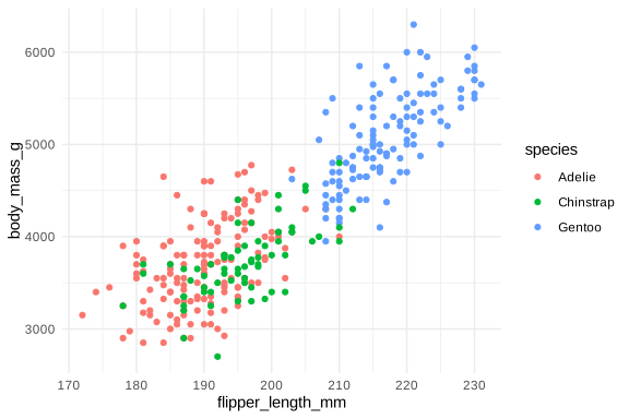
scripts/analysis.py
import framework as fwimport seaborn as snsimport statsmodels.formula.api as smf fw.scaffold() # Read a dataset from the project catalogpenguins = fw.data_read("inputs.raw.penguins")print(penguins) # Summarize, fit, and plotby_species = penguins.groupby("species").agg( n=("species", "size"), mean_mass_g=("body_mass_g", "mean"))print(by_species) formula = "body_mass_g ~ flipper_length_mm + species"model = smf.ols(formula, penguins).fit()print(model.summary()) plot = sns.scatterplot( penguins, x="flipper_length_mm", y="body_mass_g", hue="species") # Publish each onefw.publish(penguins, slug="penguins")fw.publish(by_species, slug="mass-by-species")fw.publish(model, slug="penguin-body-mass")fw.publish(plot, slug="flipper-and-mass")Data print(penguins)
       species     island  bill_length_mm  ...  body_mass_g     sex  year
0       Adelie  Torgersen            39.1  ...       3750.0    male  2007
1       Adelie  Torgersen            39.5  ...       3800.0  female  2007
2       Adelie  Torgersen            40.3  ...       3250.0  female  2007
…
[344 rows x 8 columns]
Model print(model.summary())
OLS Regression Results
Dep. Variable:            body_mass_g   R-squared: 0.783
…
                           coef    std err          t      P>|t|
----------------------------------------------------------------
Intercept            -4031.4769    584.151     -6.901      0.000
species[T.Chinstrap]  -206.5101     57.731     -3.577      0.000
species[T.Gentoo]      266.8096     95.264      2.801      0.005
flipper_length_mm       40.7054      3.071     13.255      0.000
…
print(by_species)
             n  mean_mass_g
species
Adelie     152  3700.662252
Chinstrap   68  3733.088235
Gentoo     124  5076.016260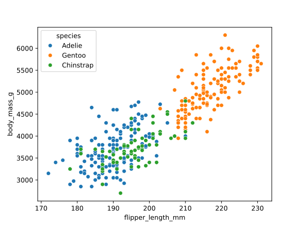
analysis.do
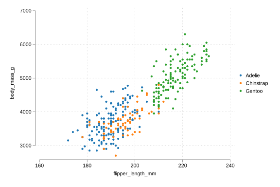
fw_project // Read a dataset from the project catalogfw_use inputs.raw.penguins, cleardestring bill_length_mm-body_mass_g, replace forceencode species, generate(species_id)list species island flipper_length_mm body_mass_g sex in 1/5 // Summarize, fit, and plottable species, statistic(frequency) /// statistic(mean body_mass_g)collect export "$fw_outputs_tables/mass-by-species.xlsx", replace regress body_mass_g flipper_length_mm i.species_id separate body_mass_g, by(species_id) veryshortlabelscatter body_mass_g? flipper_length_mm, ytitle(body_mass_g)graph export "$fw_outputs_figures/flipper-and-mass.svg", replace // Publish each onefw_publish "$fw_inputs_raw/penguins.csv", slug(penguins)fw_publish "$fw_outputs_tables/mass-by-species.xlsx", /// slug(mass-by-species)fw_publish, estimates slug(penguin-body-mass)fw_publish "$fw_outputs_figures/flipper-and-mass.svg", /// slug(flipper-and-mass)Data . list … in 1/5
     +----------------------------------------------------+
     | species      island   flippe~m   body_m~g      sex |
     |----------------------------------------------------|
  1. |  Adelie   Torgersen        181       3750     male |
  2. |  Adelie   Torgersen        186       3800   female |
  3. |  Adelie   Torgersen        195       3250   female |
…
Model . regress body_mass_g flipper_length_mm i.species_id
----------------------------------------------------------
      body_mass_g | Coefficient  Std. err.      t    P>|t|
------------------+---------------------------------------
flipper_length_mm |    40.7054    3.07102    13.25   0.000
       species_id |
       Chinstrap  |  -206.5101   57.73065    -3.58   0.000
          Gentoo  |   266.8096   95.26374     2.80   0.005
            _cons |  -4031.477   584.1513    -6.90   0.000
----------------------------------------------------------
. table species, …
-----------------------------------
            |  Frequency       Mean
------------+----------------------
  Adelie    |        152   3700.662
  Chinstrap |         68   3733.088
  Gentoo    |        124   5076.016
  Total     |        344   4201.754
-----------------------------------
Terminal
cd penguin-study # Publish files saved by any analysisfw publish inputs/raw/penguins.csv --slug penguinsfw publish outputs/tables/mass-by-species.csvfw publish outputs/models/penguin-body-mass.jsonfw publish outputs/figures/flipper-and-mass.svgPublishing penguins.csv, 15 KB, to this project on framework.pub.
Upload it? [y/N] y
Published penguins, version 1.
Link: https://framework.pub/@examples/penguin-study/penguins
…
Published mass-by-species, version 1.
…
Published penguin-body-mass, version 1.
…
Published flipper-and-mass, version 1.
Link: https://framework.pub/@examples/penguin-study/flipper-and-massConnect to Framework Cloud to reuse project settings and publish updates at the same link.
Framework keeps your project structured from start to finish
Start the project, run the analysis, and publish the results with one folder layout, one data catalog, and one set of settings.
01
Start your project
Build a project from trusted blueprints. Catalog your data, manage package dependencies, set safety guidelines, configure Quarto or Jupyter notebooks, and set up database connections in one place. Signed in to Framework Cloud, a new project starts from your saved blueprint.
framework::new_project("penguin-study") # Signed in to Framework Cloud, the project starts# from your saved blueprint: its folders, package# list, and notebook settings. Open the files to see them. # Or use a project created in Cloudframework::new_project(key = "<project token>")framework.new_project("penguin-study") # Signed in to Framework Cloud, the project starts# from your saved blueprint: its folders, package# list, and notebook settings. Open the files to see them. # Or use a project created in Cloudframework.new_project(key="<project token>")fw new penguin-study # Or create the repository on GitHubfw new penguin-study --github username/penguin-studyscripts/install-packages.R
# Install packages declared in settings/packages.yml.# Session setup and attachment happen later in scaffold().framework::packages_install()scripts/analysis.R
# Apply the configured seed and ggplot theme.framework::scaffold()scripts/data.R
# Resolve the catalog name and record the file hash.penguins <- data_read("inputs.raw.penguins")scripts/data.R
measurements <- db_query( "SELECT species, island FROM field_measurements", "study_db")scripts/install-packages.py
import framework # Install dependencies declared in pyproject.toml.# Uses uv sync when uv is available.framework.packages_install()scripts/analysis.py
import framework # Apply the configured seed and prepare helper imports.framework.scaffold()scripts/data.py
# Resolve the catalog name and record the file hash.penguins = fw.data_read("inputs.raw.penguins")scripts/data.py
measurements = fw.db_query( "SELECT species, island FROM field_measurements", "study_db")02
Conduct your analysis
Load your project settings and helper functions, read data by its catalog name, and check whether an input has changed.
library(framework) # Load all files in functions/.# Apply the configured ggplot theme.scaffold() # Read the input and record its hashpenguins <- data_read("inputs.raw.penguins")penguins <- drop_incomplete(penguins)model <- lm(body_mass_g ~ flipper_length_mm + species, penguins)plot <- ggplot(penguins, aes(flipper_length_mm, body_mass_g)) + geom_point() # Verify that the input is unchangeddata_verify("inputs.raw.penguins")import framework as fwimport statsmodels.formula.api as smfimport matplotlib.pyplot as plt fw.scaffold()from data_prep import drop_incomplete # Read the input and record its hashpenguins = fw.data_read("inputs.raw.penguins")penguins = drop_incomplete(penguins)model = smf.ols( "body_mass_g ~ flipper_length_mm + species", penguins).fit()fig, ax = plt.subplots()ax.scatter(penguins["flipper_length_mm"], penguins["body_mass_g"]) # Verify that the input is unchangedfw.data_verify("inputs.raw.penguins")functions/data_prep.R
# Sourced by scaffold()drop_incomplete <- function(data) { # Keep penguins with every measurement data[complete.cases(data), ]}functions/data_prep.py
# Importable after fw.scaffold()def drop_incomplete(data): # Keep penguins with every measurement return data.dropna()03
Publish your work
Publish a model from your script and share its link. Publish again with the same slug and collaborators get the latest version at that link.
publish(model, slug = "penguin-body-mass")fw.publish(model, slug="penguin-body-mass")fw_publish, estimates slug(penguin-body-mass)fw publish outputs/models/penguin-body-mass.jsonPenguin body mass model Version 2
R · lm() · body_mass_g ~ flipper_length_mm + species
Python · statsmodels OLS · body_mass_g ~ flipper_length_mm + species
Stata · regress · regress body_mass_g flipper_length_mm i.species_id
R · lm(), saved as JSON · body_mass_g ~ flipper_length_mm + species
| Term | Estimate | Std. error | p-value |
|---|---|---|---|
| (Intercept) | −4031.477 | 584.151 | <0.001 |
| flipper_length_mm | 40.705 | 3.071 | <0.001 |
| speciesChinstrap | −206.510 | 57.731 | <0.001 |
| speciesGentoo | 266.810 | 95.264 | 0.005 |
> summary(model)
…
Coefficients:
                   Estimate Std. Error t value Pr(>|t|)
(Intercept)       -4031.477    584.151  -6.901 2.55e-11 ***
flipper_length_mm    40.705      3.071  13.255  < 2e-16 ***
speciesChinstrap   -206.510     57.731  -3.577 0.000398 ***
speciesGentoo       266.810     95.264   2.801 0.005392 **
---
Multiple R-squared:  0.7826,	Adjusted R-squared:  0.7807
…| Term | Estimate | Std. error | p-value |
|---|---|---|---|
| (Intercept) | −4031.477 | 584.151 | <0.001 |
| species[T.Chinstrap] | −206.510 | 57.731 | <0.001 |
| species[T.Gentoo] | 266.810 | 95.264 | 0.005 |
| flipper_length_mm | 40.705 | 3.071 | <0.001 |
>>> print(model.summary())
OLS Regression Results
Dep. Variable:            body_mass_g   R-squared: 0.783
…
                           coef    std err          t      P>|t|
----------------------------------------------------------------
Intercept            -4031.4769    584.151     -6.901      0.000
species[T.Chinstrap]  -206.5101     57.731     -3.577      0.000
species[T.Gentoo]      266.8096     95.264      2.801      0.005
flipper_length_mm       40.7054      3.071     13.255      0.000
…| Term | Estimate | Std. error | p-value |
|---|---|---|---|
| flipper_length_mm | 40.705 | 3.071 | <0.001 |
| 2.species_id | −206.510 | 57.731 | <0.001 |
| 3.species_id | 266.810 | 95.264 | 0.005 |
| (Intercept) | −4031.477 | 584.151 | <0.001 |
. regress body_mass_g flipper_length_mm i.species_id
…
    Residual |  47666988.2       338  141026.592   R-squared       =    0.7826
----------------------------------------------------------
      body_mass_g | Coefficient  Std. err.      t    P>|t|
------------------+---------------------------------------
flipper_length_mm |    40.7054    3.07102    13.25   0.000
       species_id |
       Chinstrap  |  -206.5101   57.73065    -3.58   0.000
          Gentoo  |   266.8096   95.26374     2.80   0.005
            _cons |  -4031.477   584.1513    -6.90   0.000
----------------------------------------------------------| Term | Estimate | Std. error | p-value |
|---|---|---|---|
| (Intercept) | −4031.477 | 584.151 | <0.001 |
| flipper_length_mm | 40.705 | 3.071 | <0.001 |
| speciesChinstrap | −206.510 | 57.731 | <0.001 |
| speciesGentoo | 266.810 | 95.264 | 0.005 |
$ cat outputs/models/penguin-body-mass.json
{
  "schema": "framework.artifact/v1",
  "kind": "model",
  "source": {"language": "r", "class": ["lm"]},
  "formula": "body_mass_g ~ flipper_length_mm + species",
  "tables": [{"title": "Coefficients", "rows": [
    ["(Intercept)", -4031.47689069363, 584.151339929479, …],
    ["flipper_length_mm", 40.7054007772805, 3.07101973140904, …],
  …
Framework Cloud
Framework Cloud is a companion web app for Framework. It stores your project defaults, blueprints, AI skills, and other settings. It also lets you share your work securely.
Use it for free at framework.pub or host it on your own server.
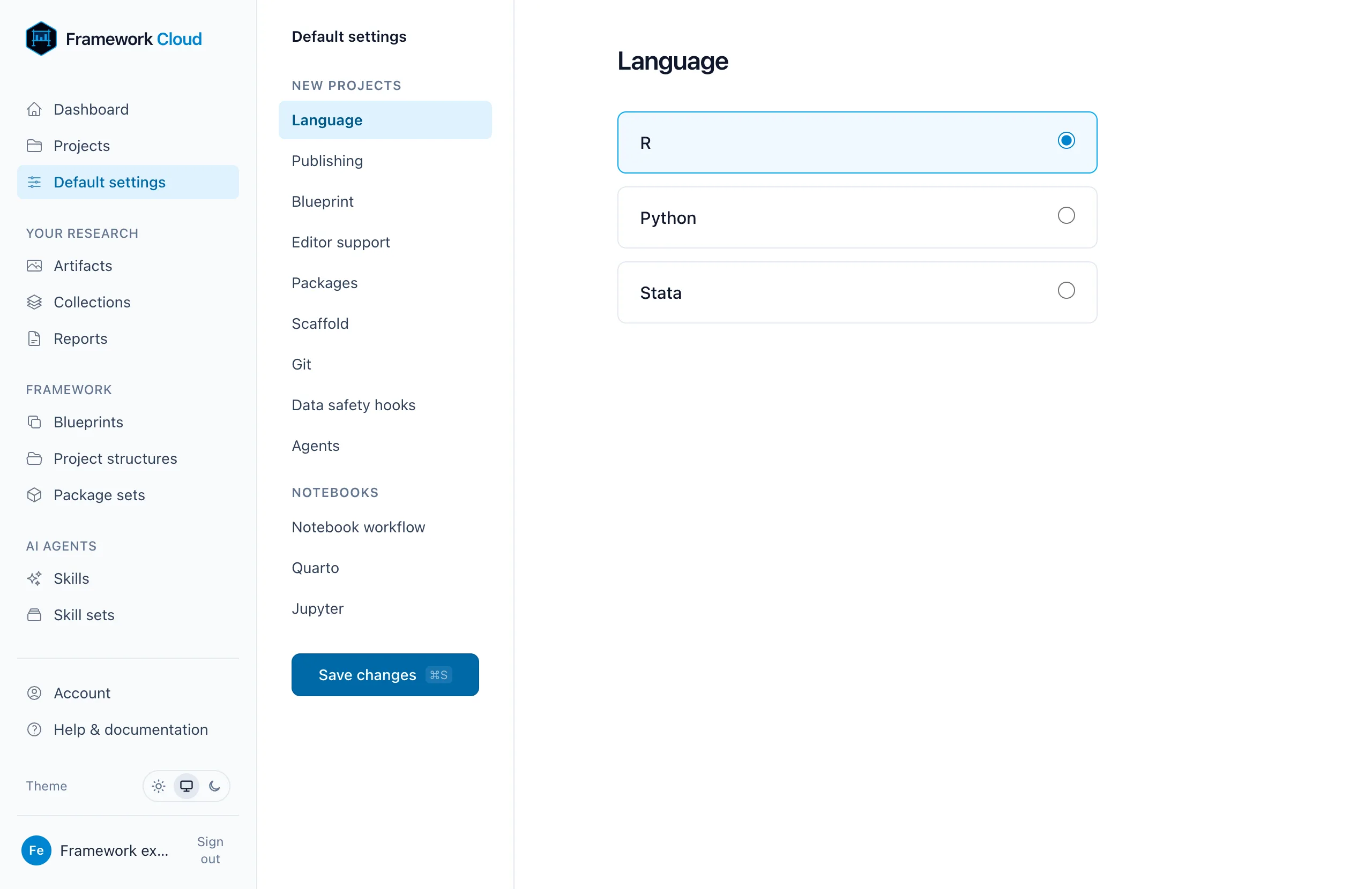
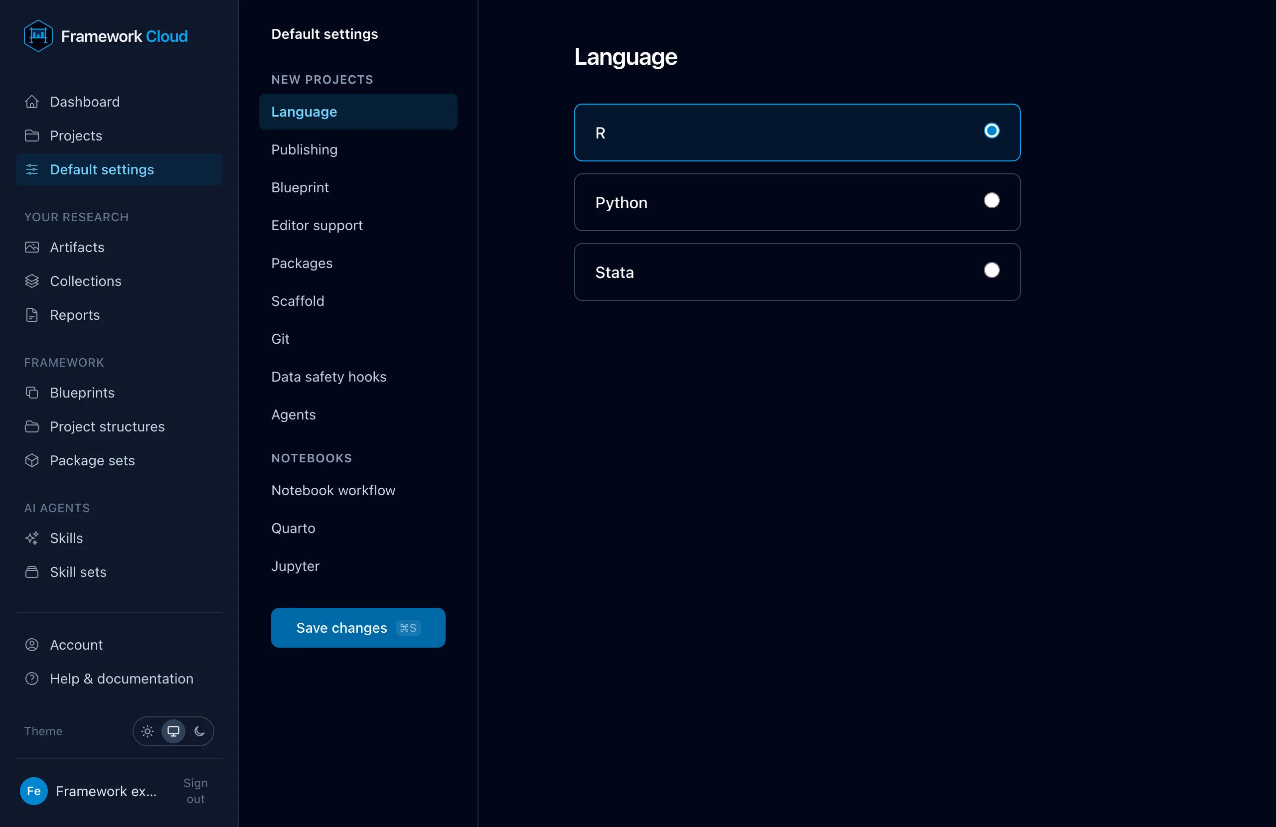
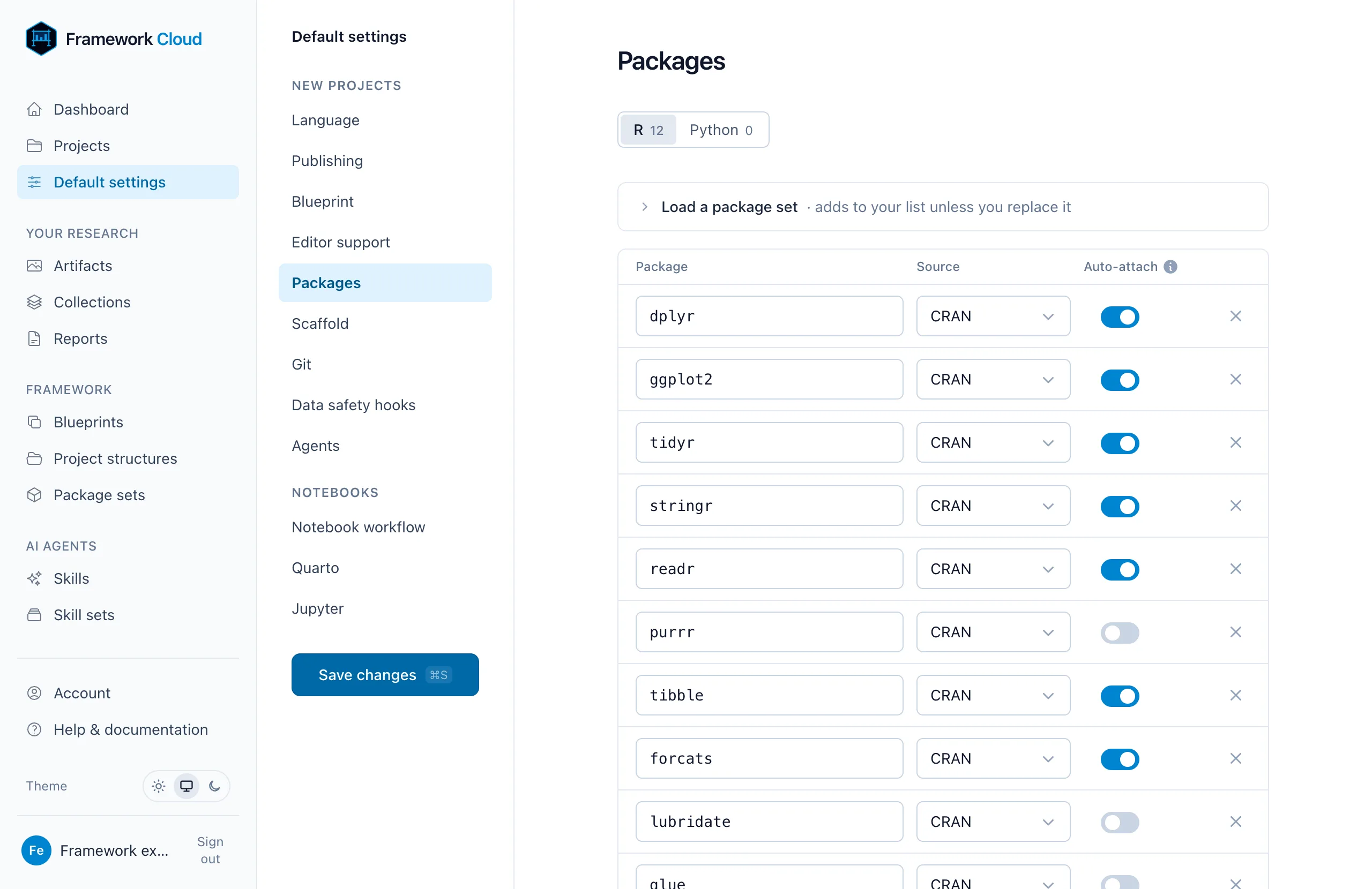
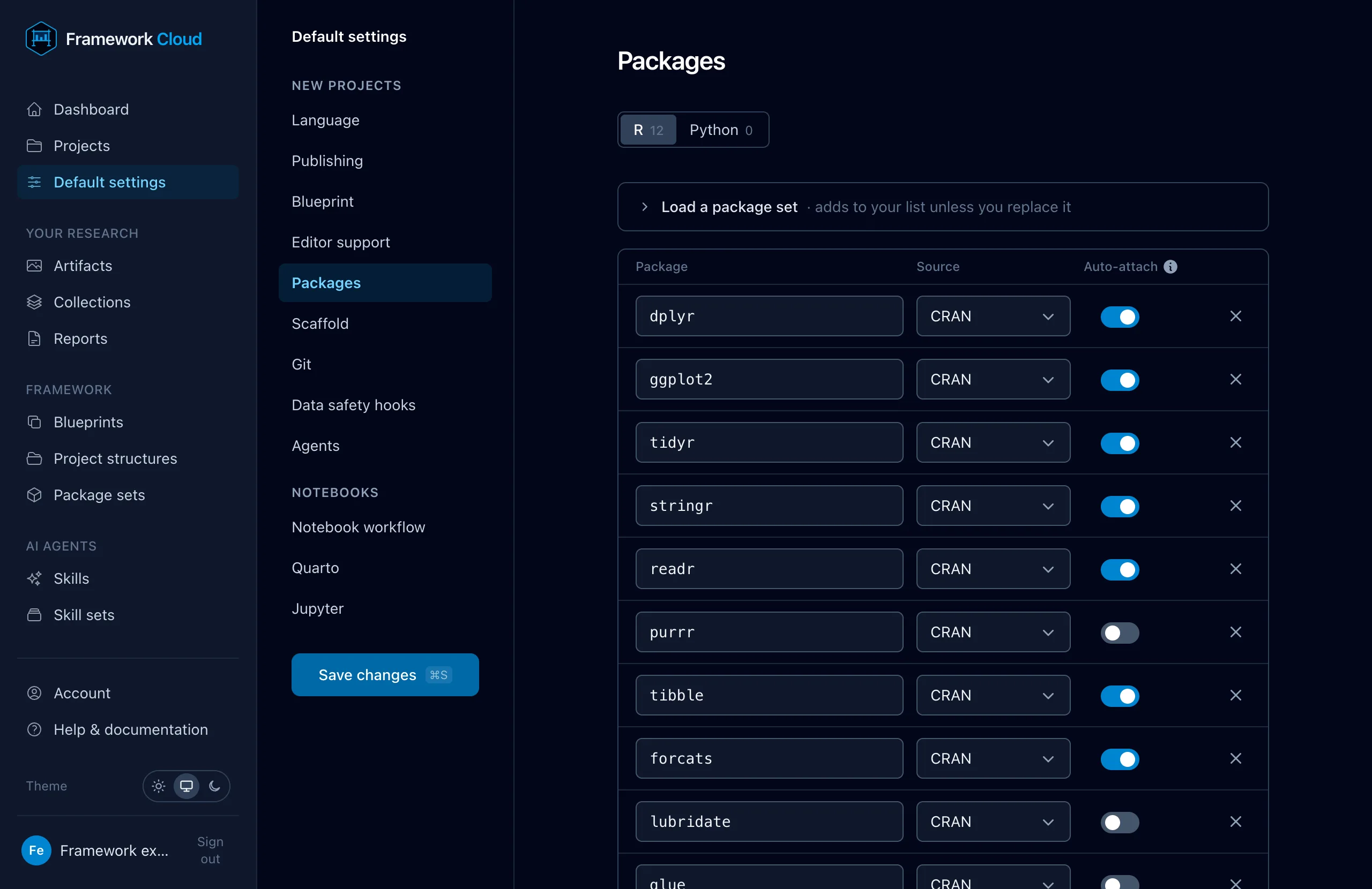
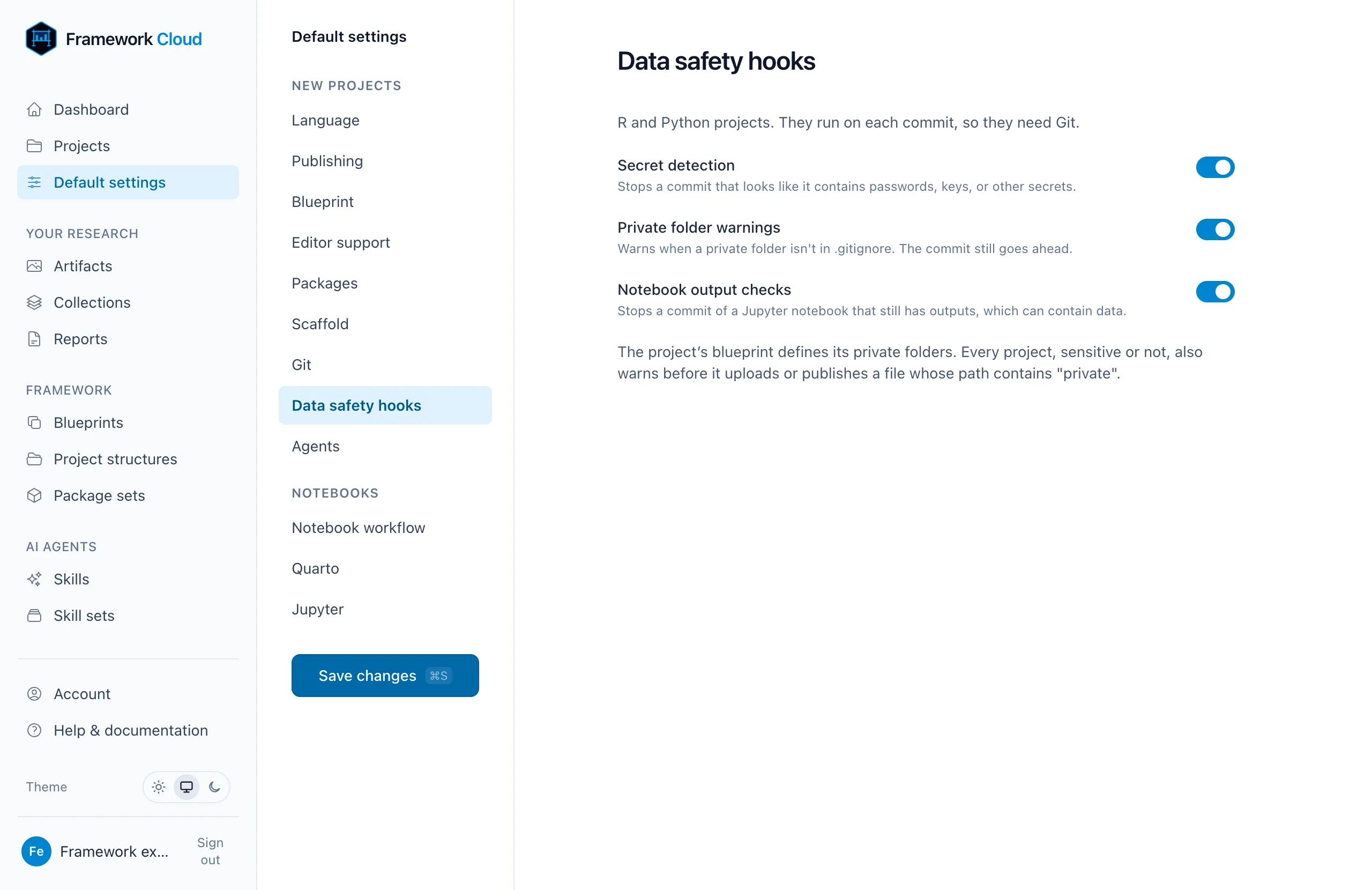
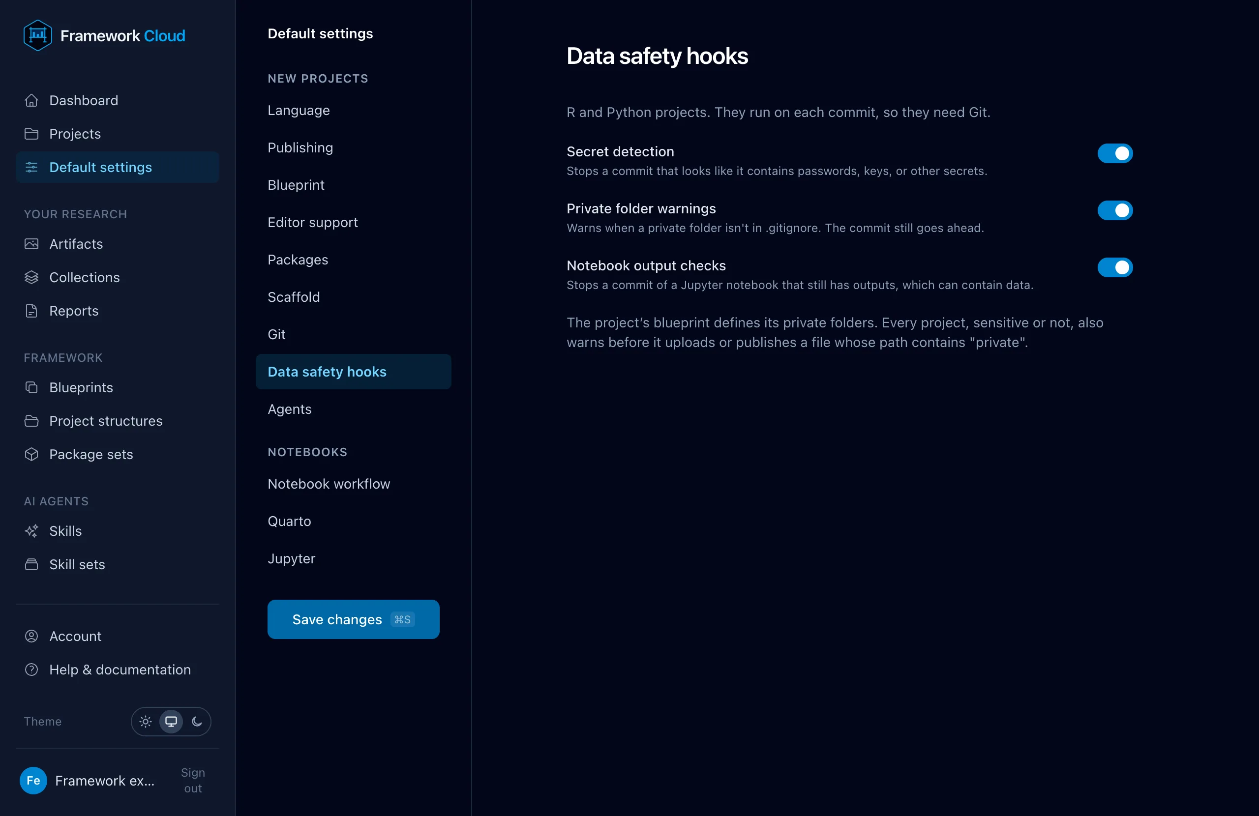
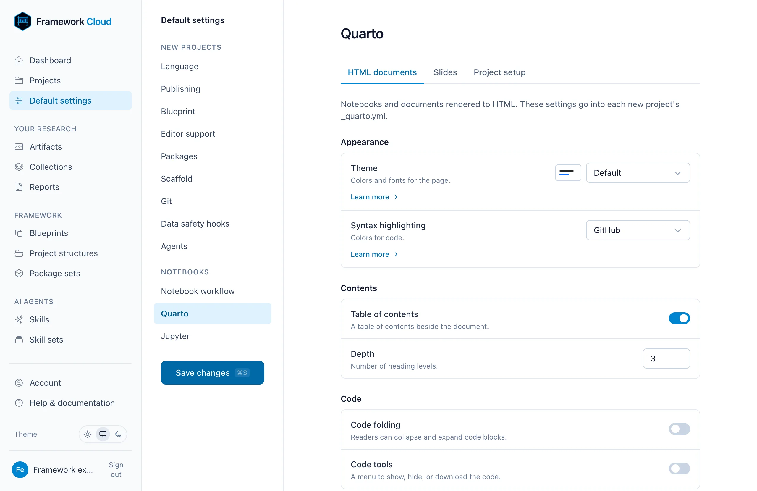
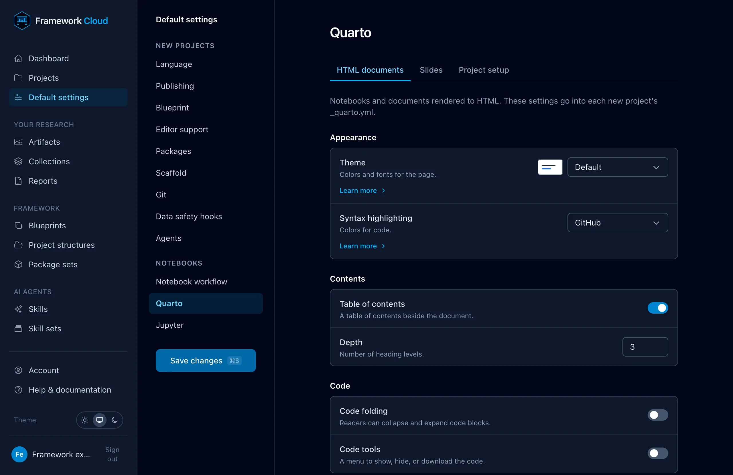
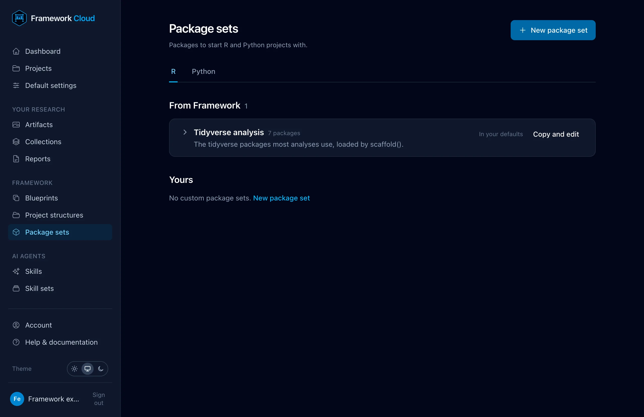
Choose R, Python, or Stata for new projects.Pick the packages every new project installs.Stop commits that contain secrets, private folders, or notebook outputs.Set the theme, contents, and code options for documents.
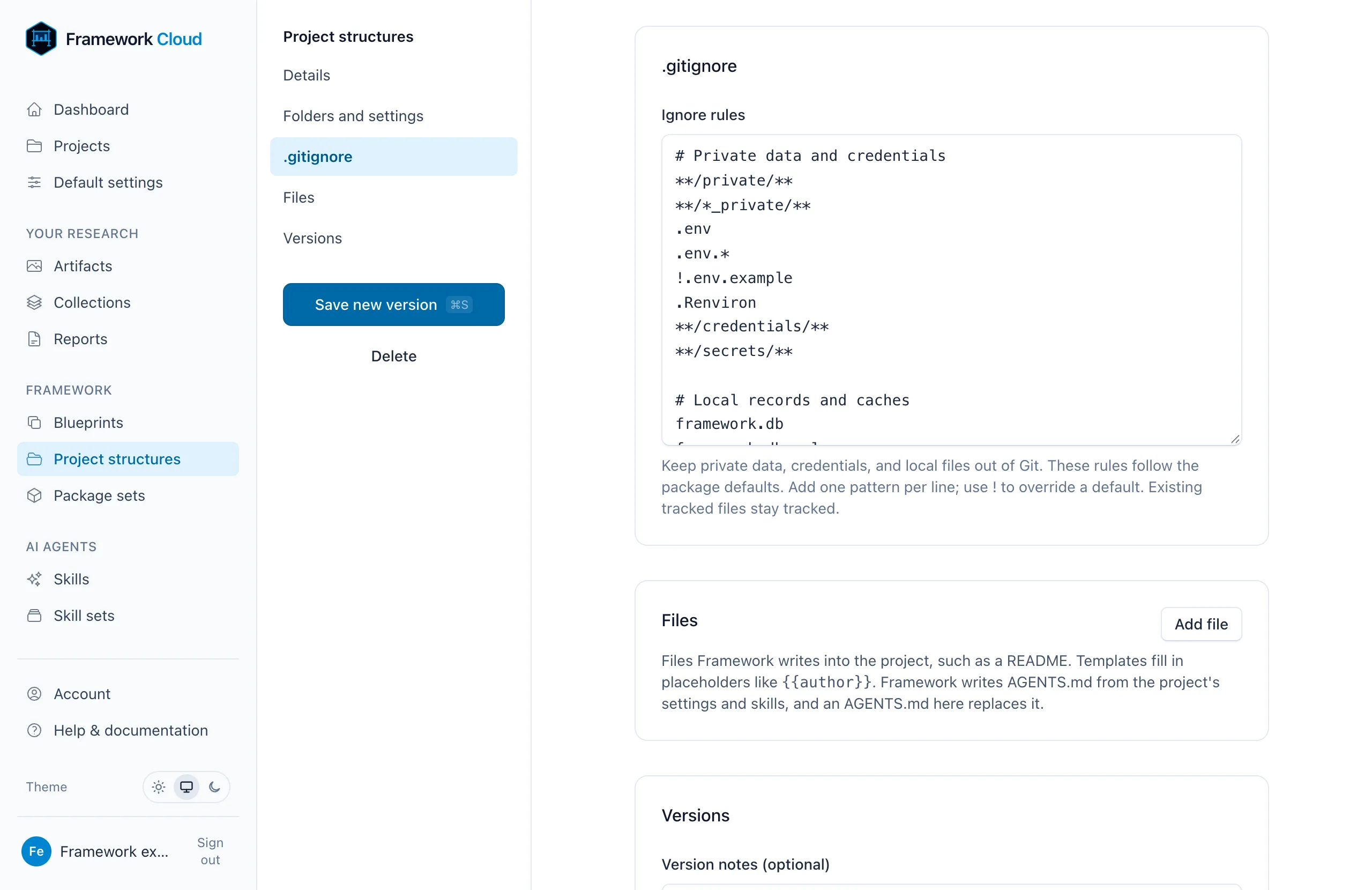
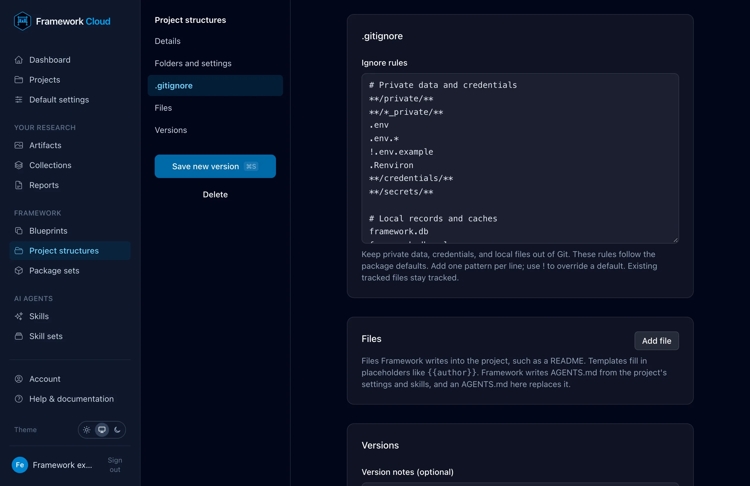
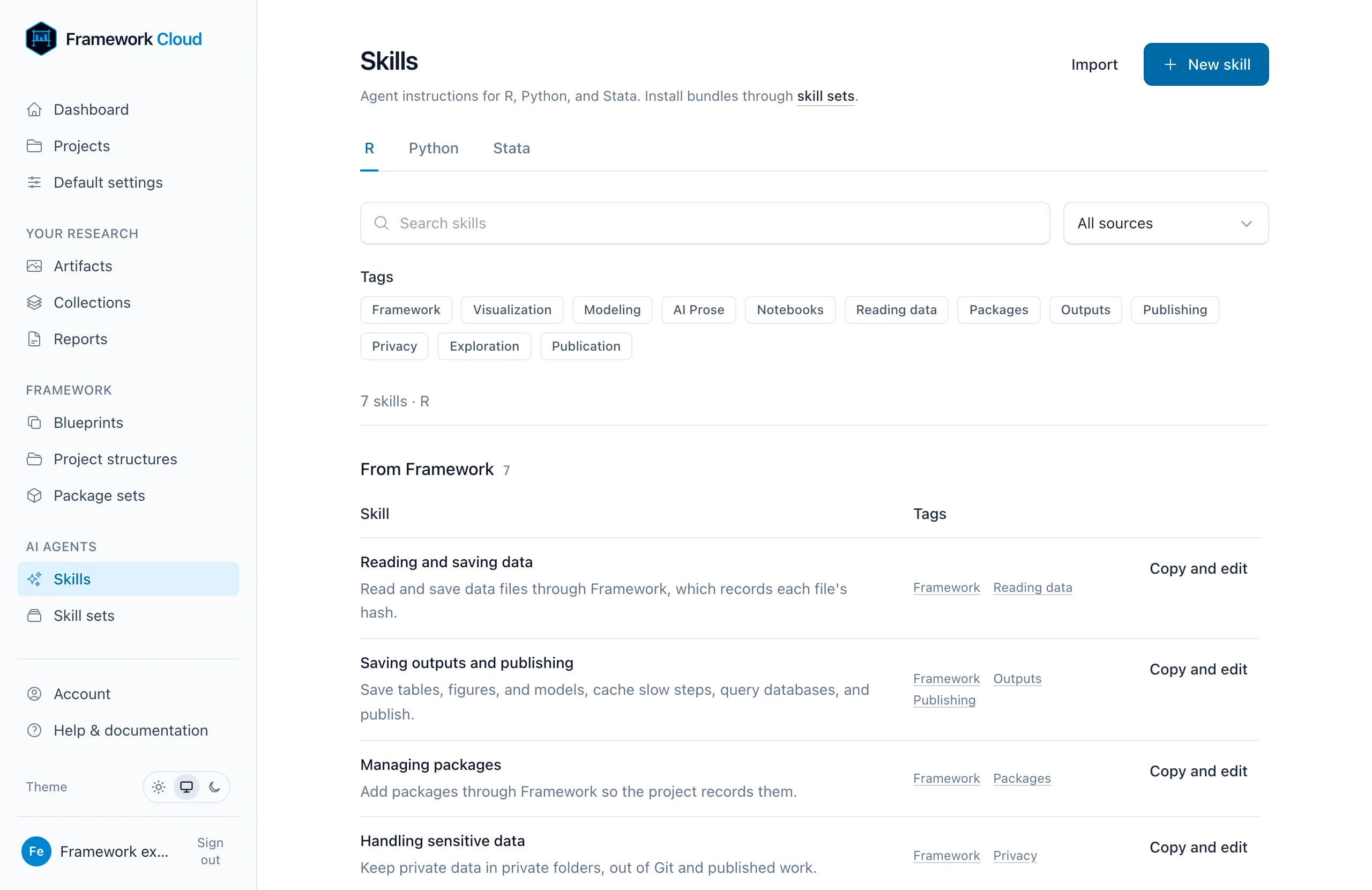
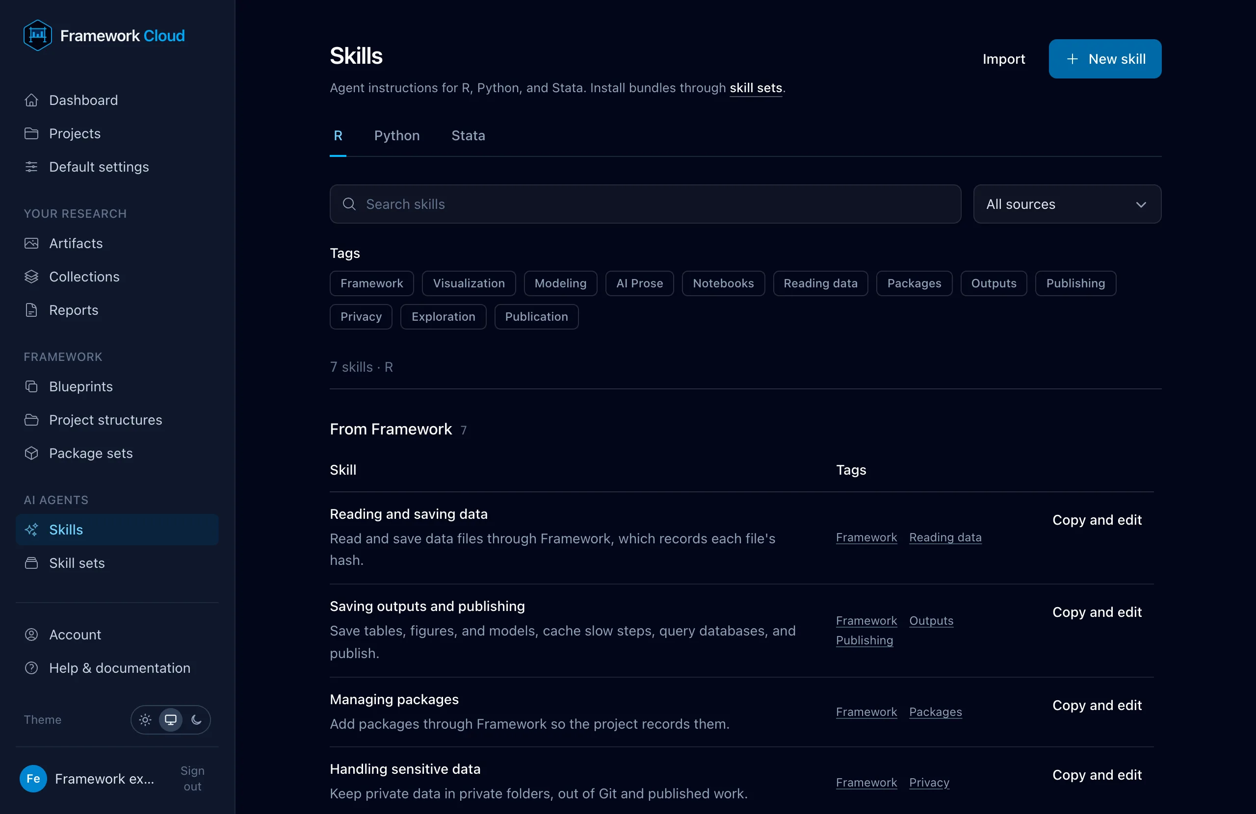
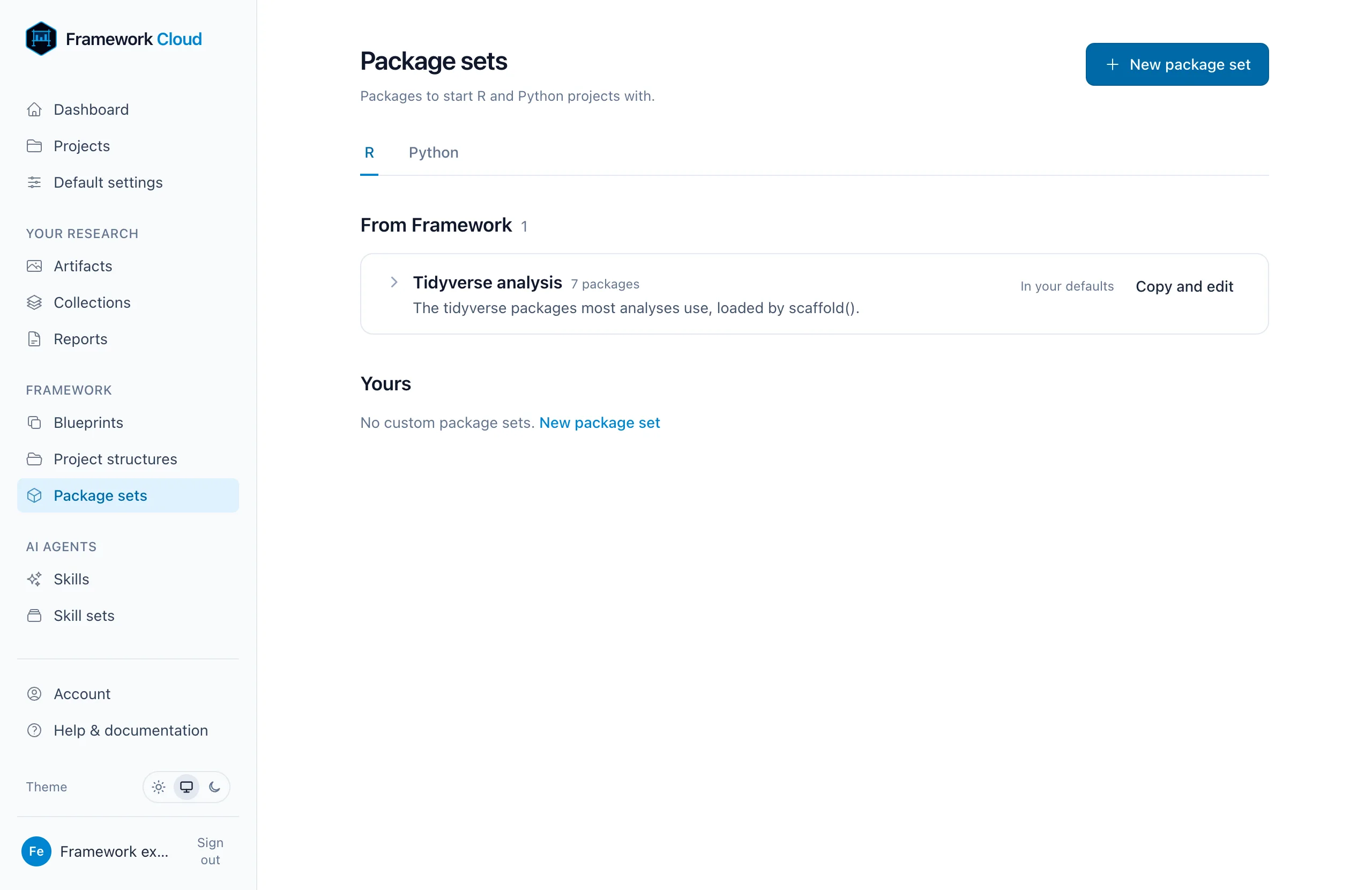
Edit the rules that keep private data out of Git.Copy, edit, or import the skills your AI agent uses.Group packages you use together and add them in one step.
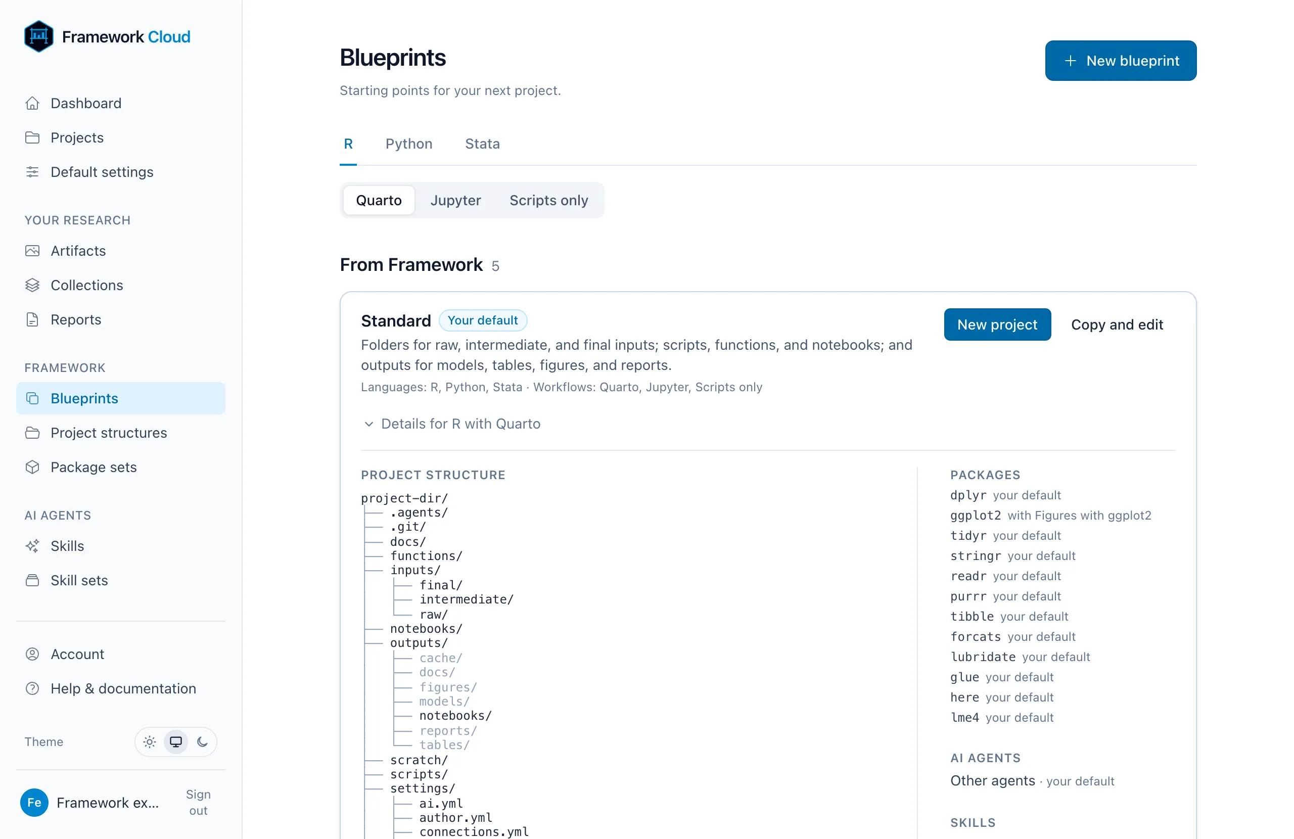
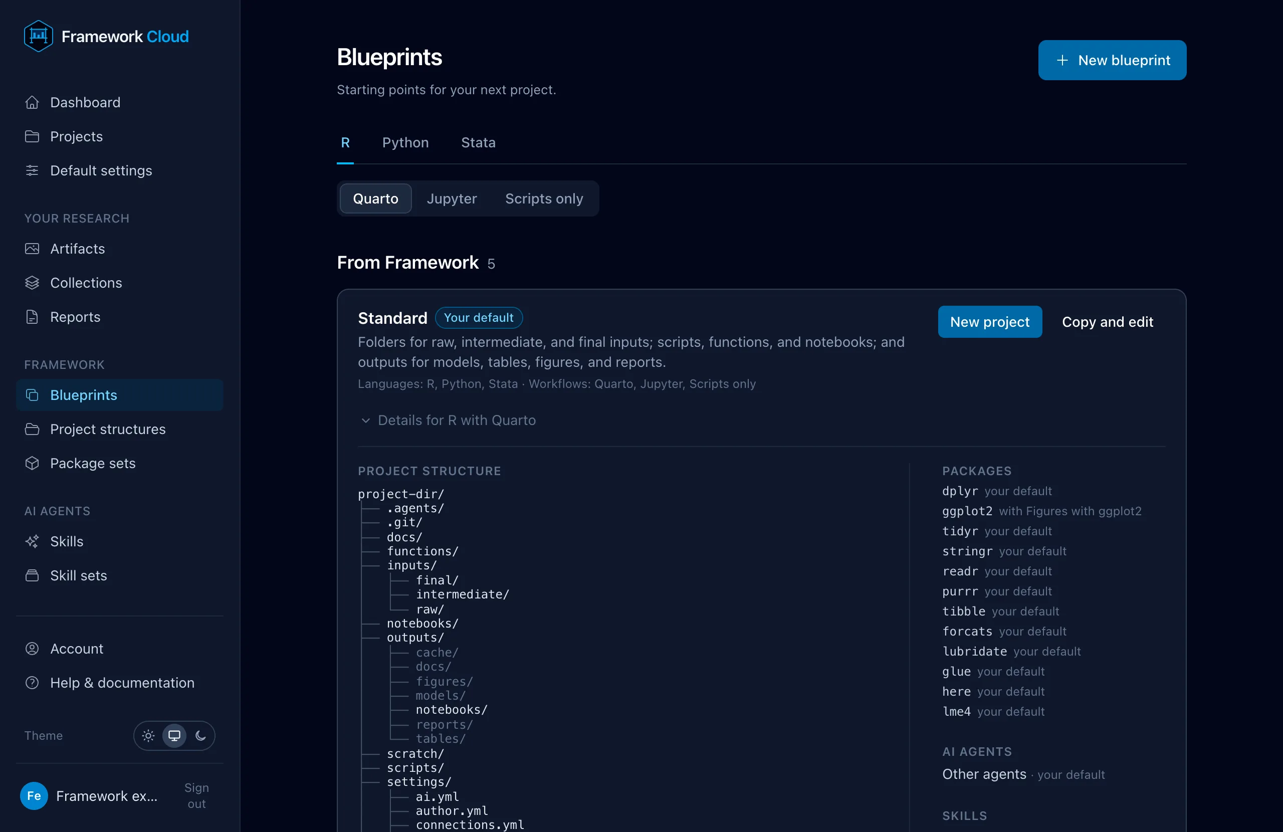
Combine a structure, packages, and skills into a starting point.
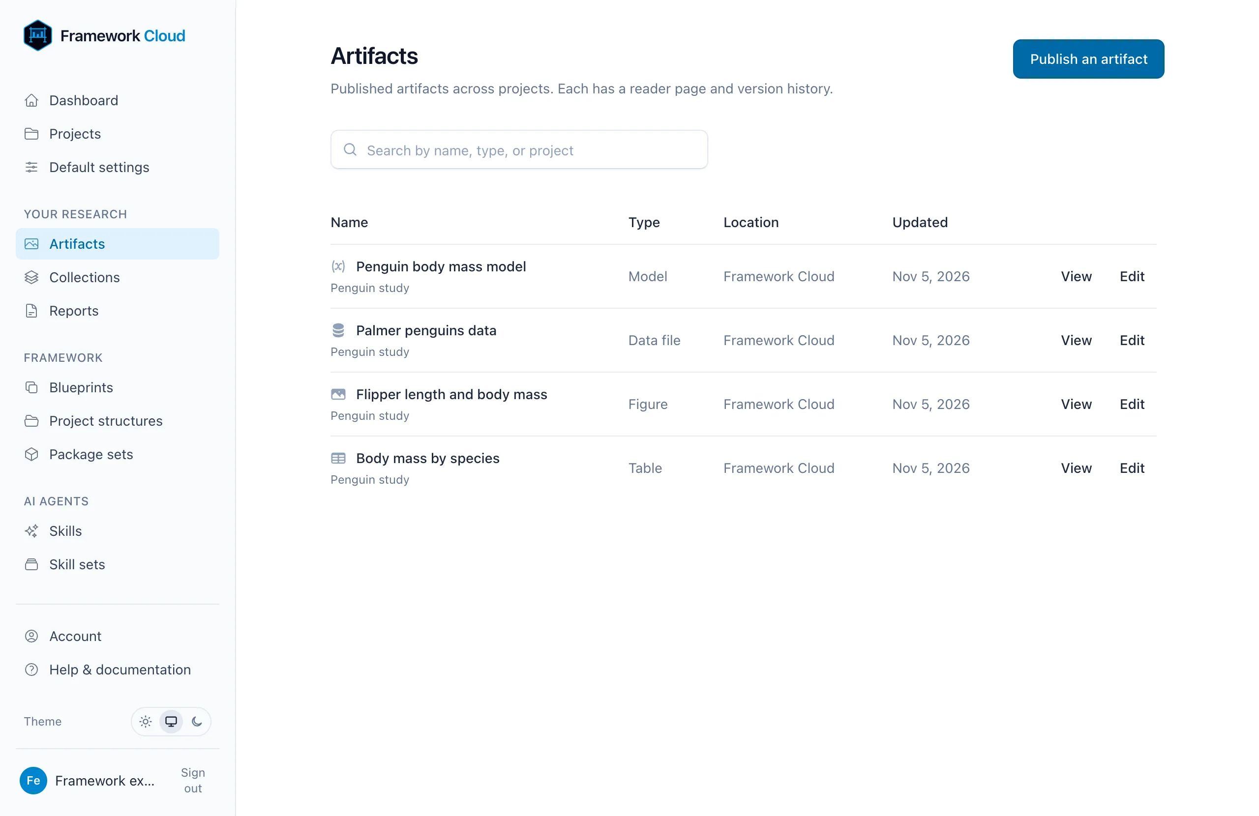
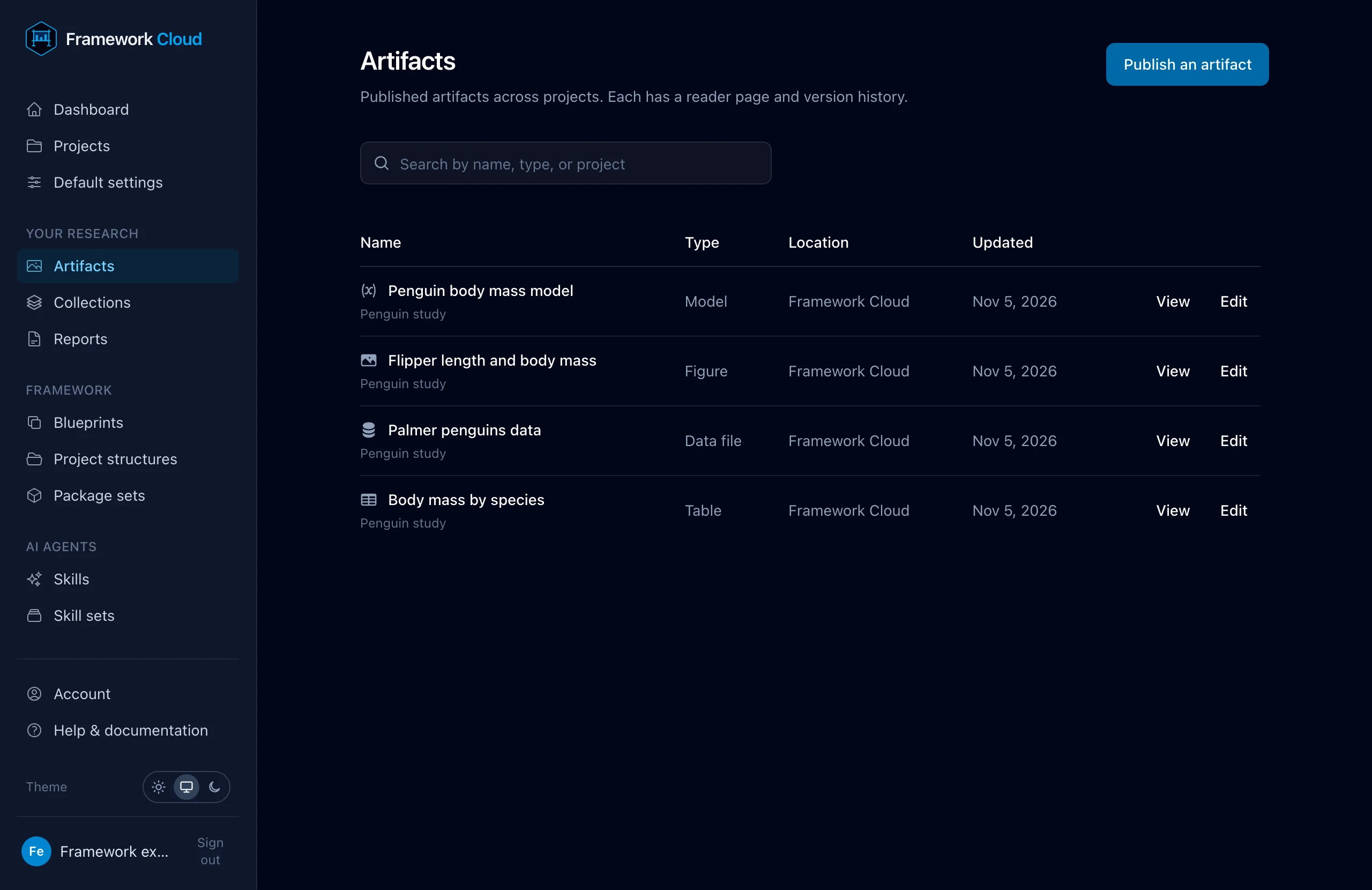
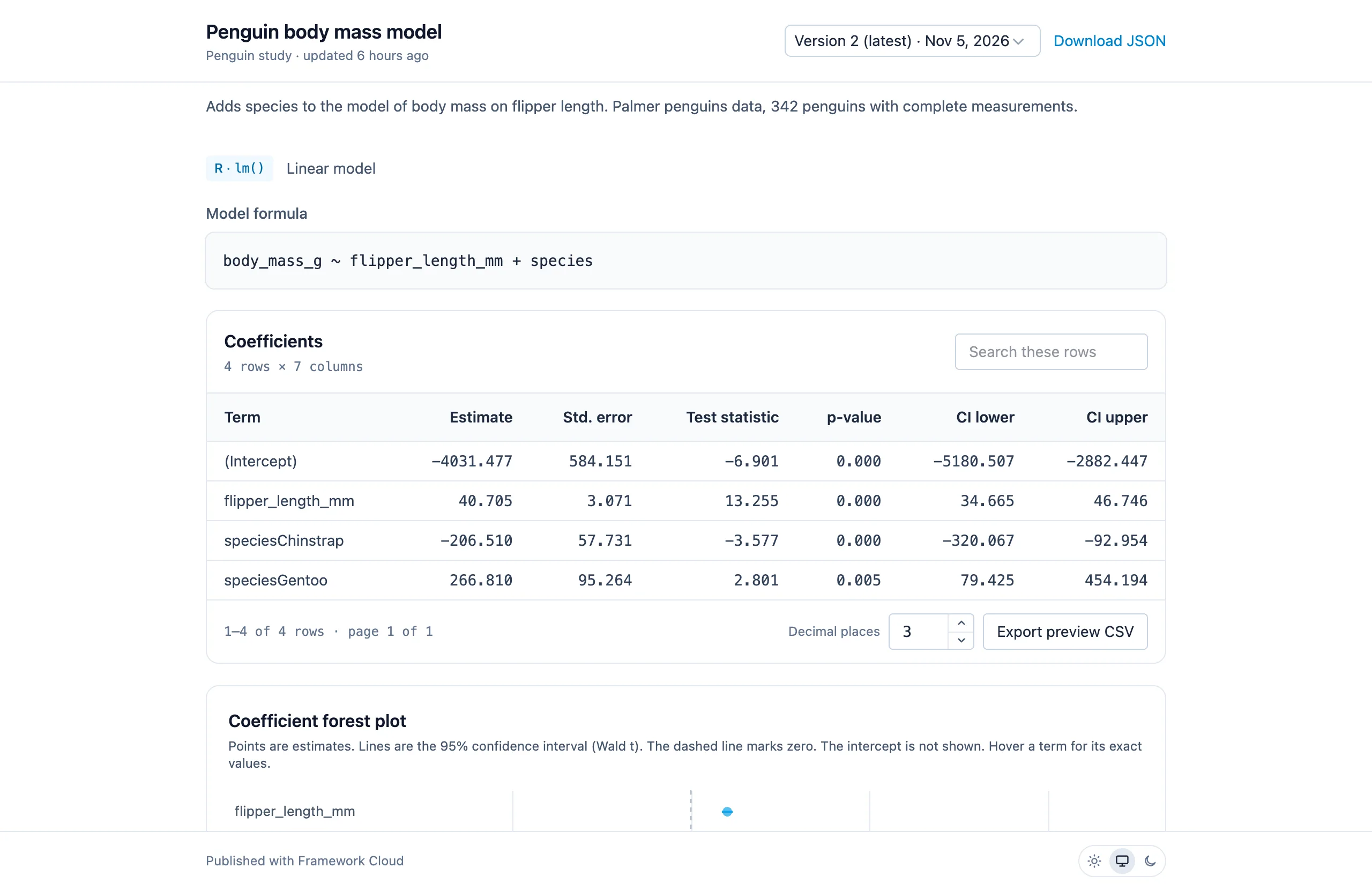
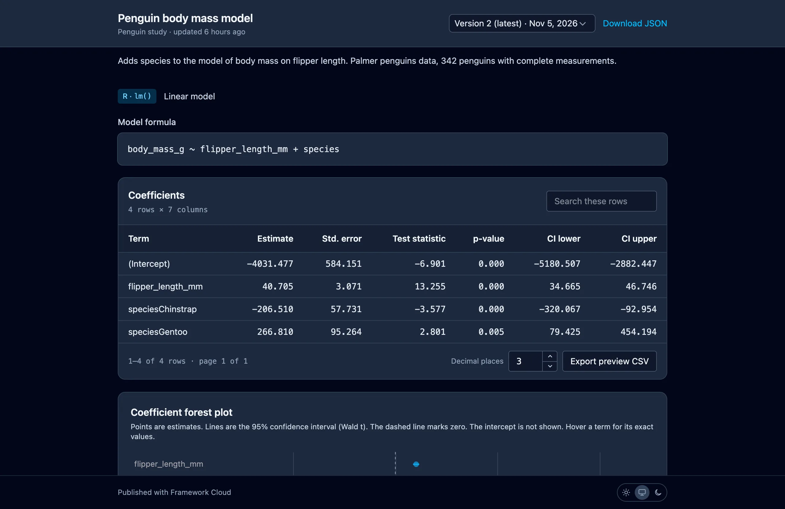
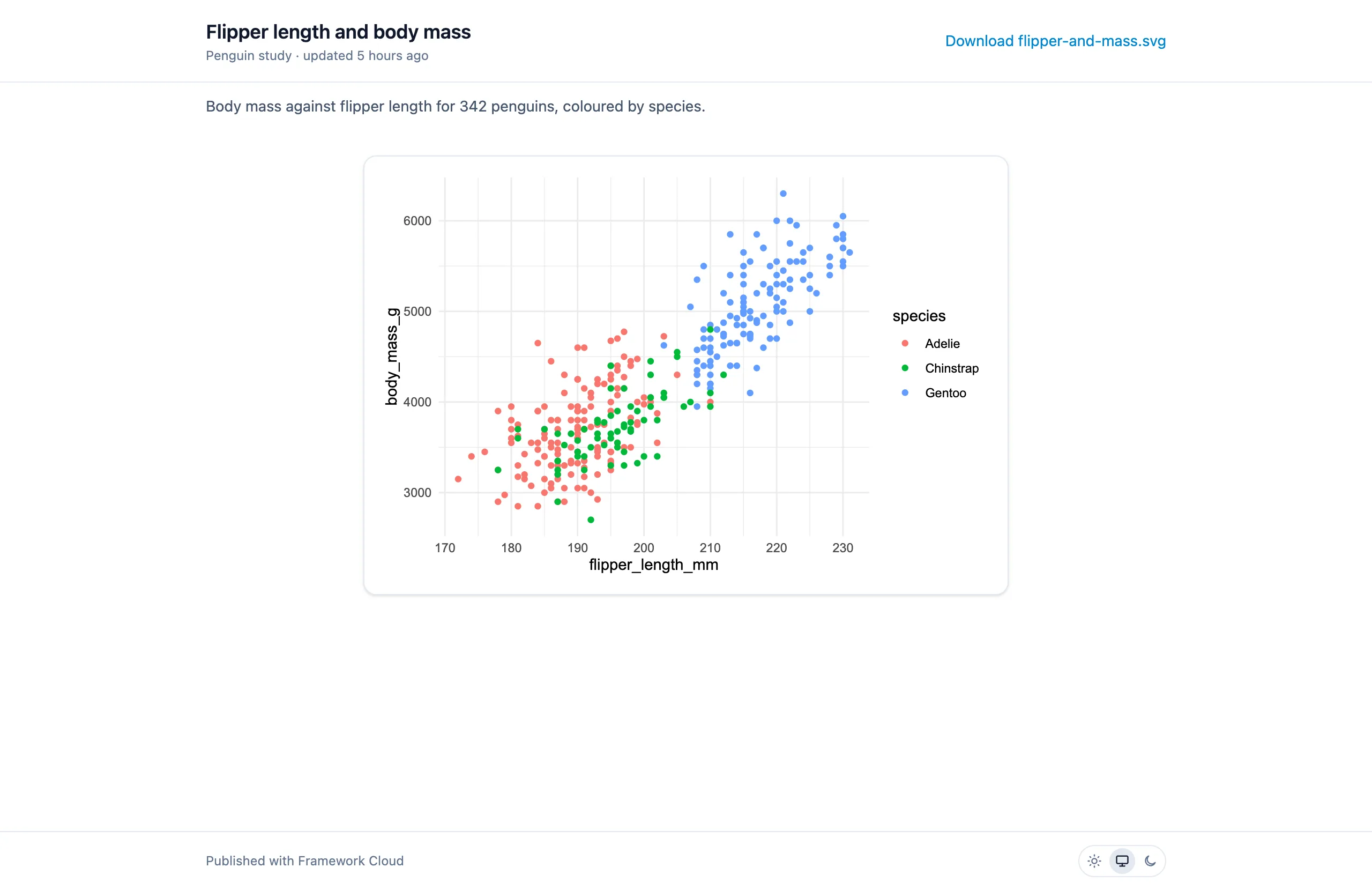
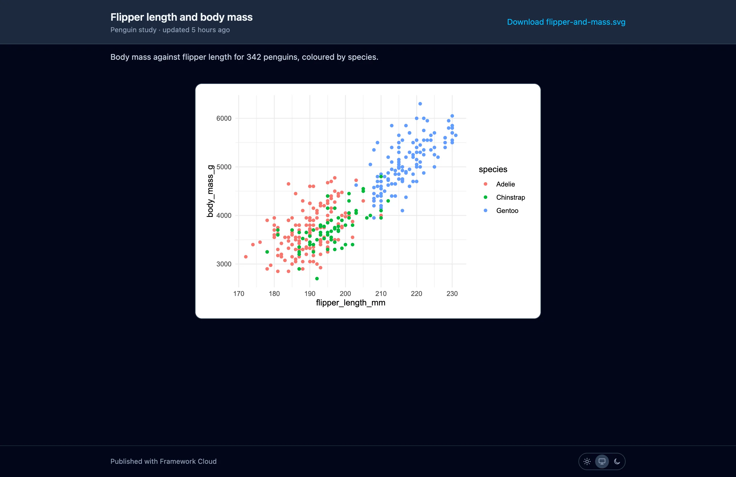
Find everything you have published, across projects.Readers get a formatted, searchable model summary.Readers see the figure and can download the file.
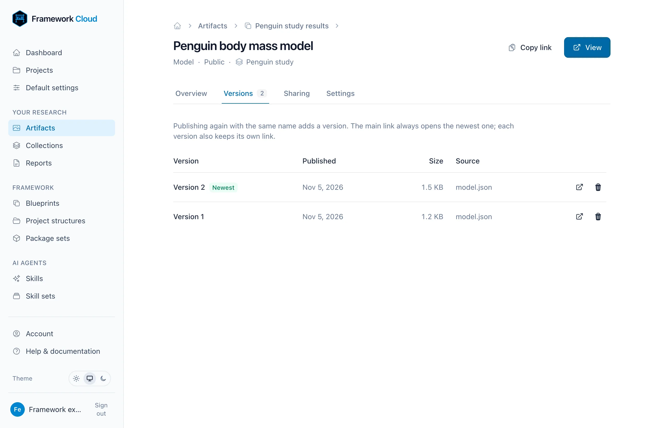
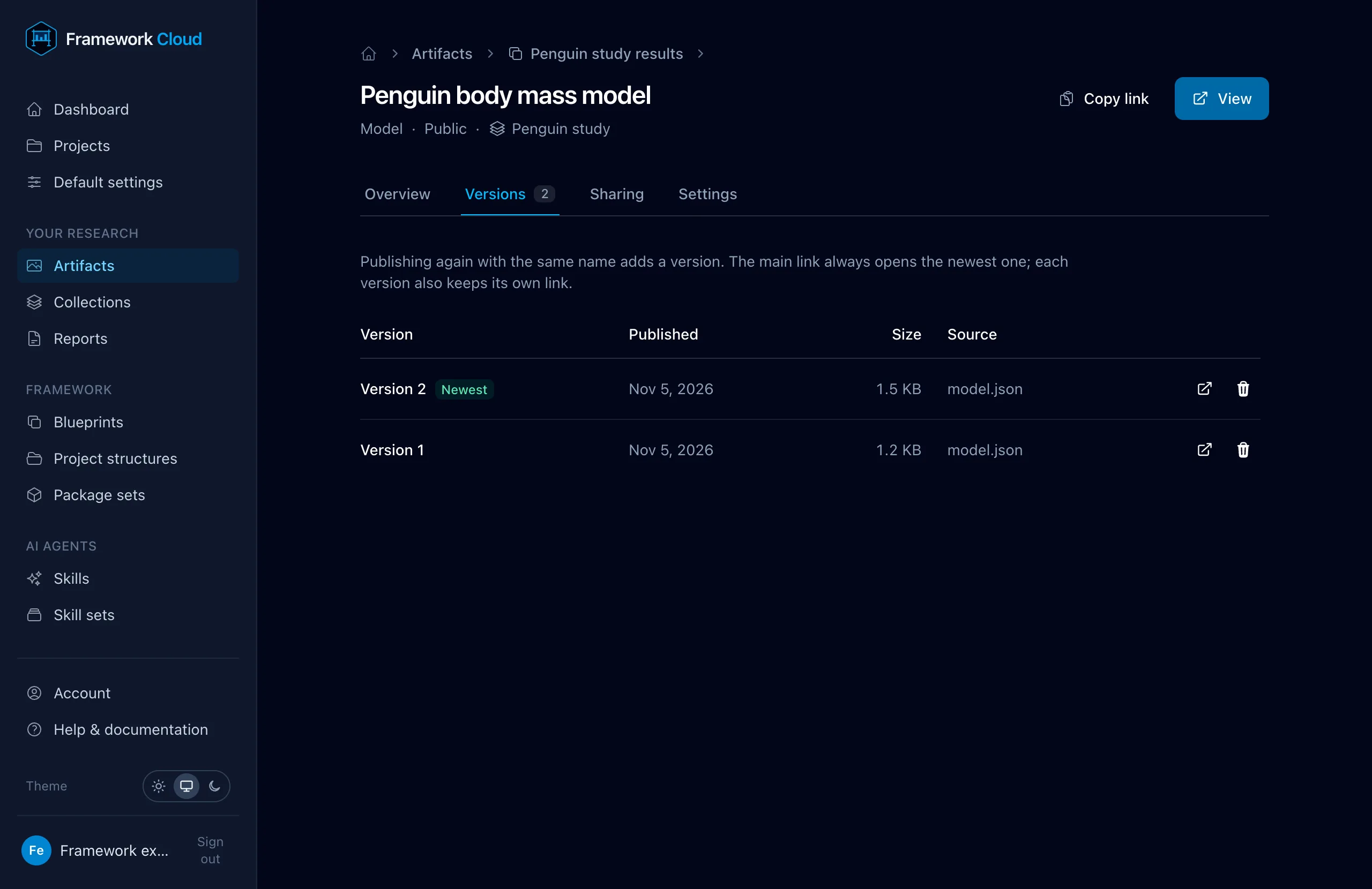
Open any earlier version. The main link shows the newest.
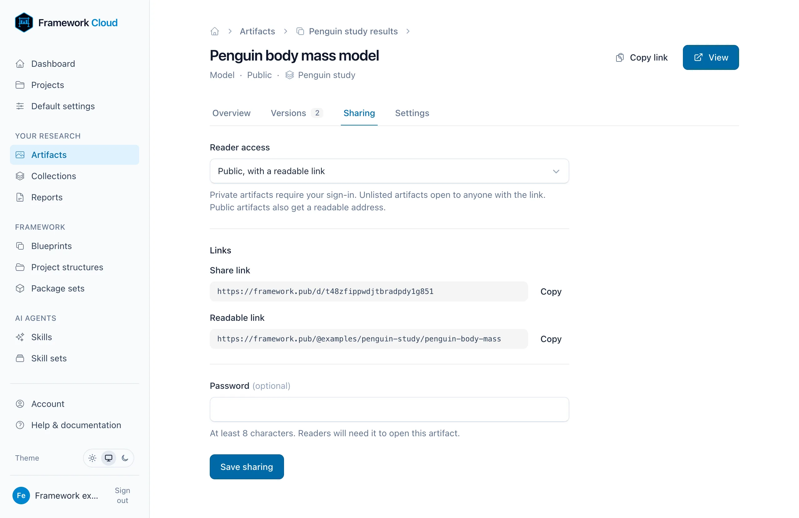
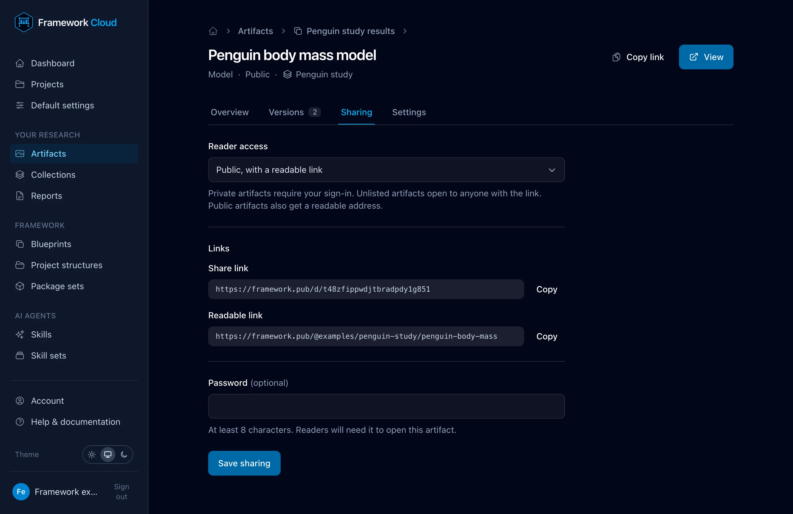
Choose who can read it, copy its links, or add a password.
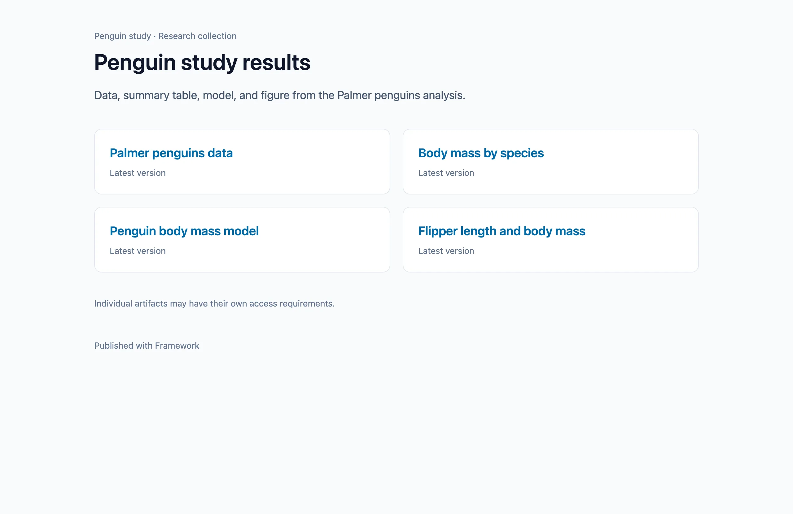
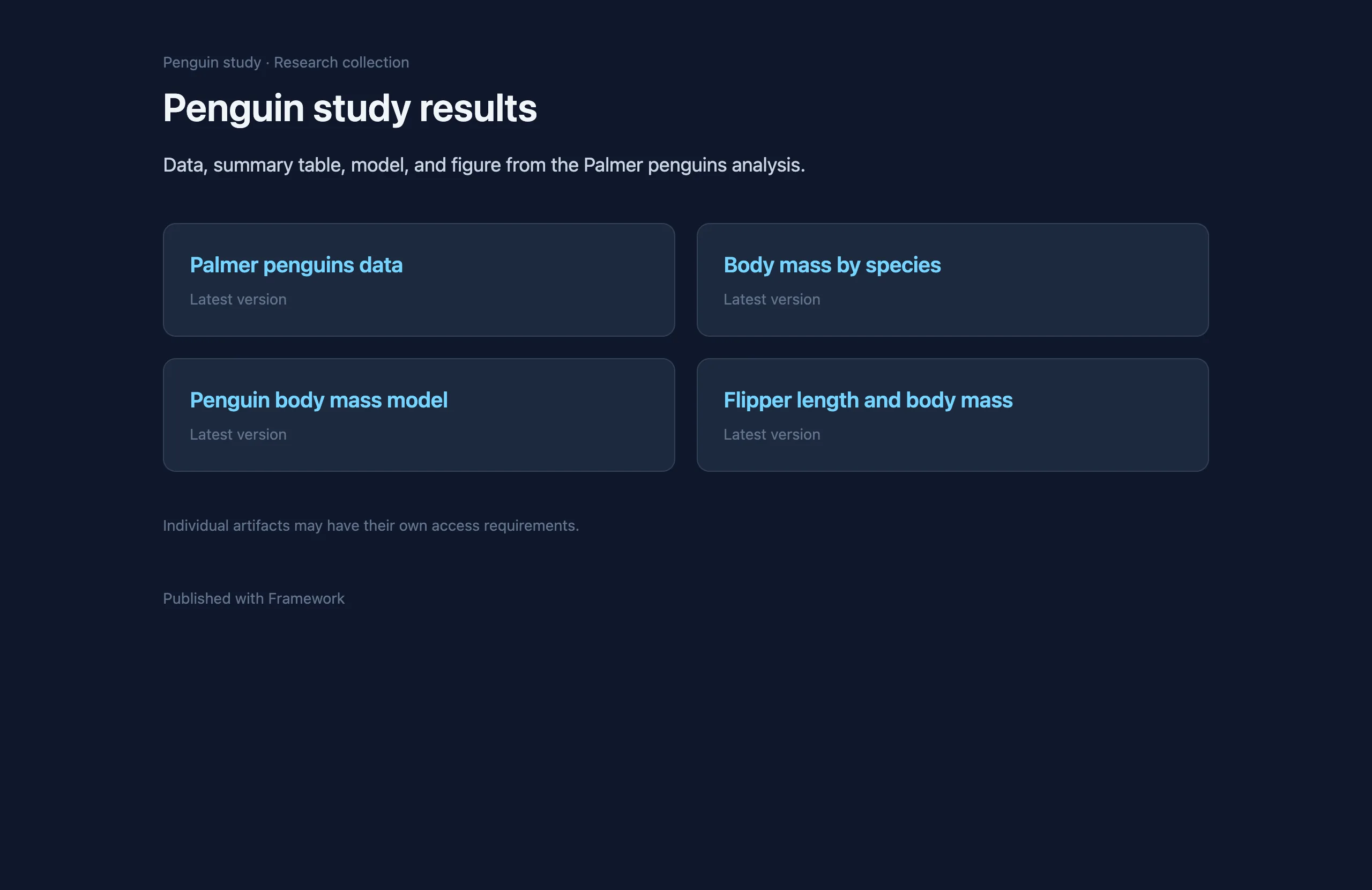
Share one link for a set of related results.
Data security and integrity
Framework keeps private data out of Git, guards inputs against accidental changes, and records fingerprints you can show collaborators and reviewers.
Explicit private directories
Keep sensitive inputs and unreviewed outputs in private/ directories. Put reviewed results in public/ directories when they are ready to share.
Git safeguards
Each structure has an editable .gitignore template. Optional pre-commit checks catch private data and missing ignore rules before a commit.
File fingerprints
data_read() records input hashes and warns when data changes. Lock inputs to stop changed files from being read, and check them with data_verify().
Data verification ledger
Share input fingerprints and verification metadata through Framework Cloud for transparency. Your datasets stay on your machine.
$ git add inputs/private/raw/penguins.csv$ git commit -m "Add study data" ✗ FAIL: gitignore coverage (2 issues)✗ FAIL: private data exposure (1 issue)... inputs/private/raw/penguins.csv Reason: Private data file not in .gitignore...✗ AUDIT FAILED - Critical security issues found✗ Data security check failed $ git add inputs/private/raw/penguins.csv$ git commit -m "Add study data" ✗ FAIL: gitignore coverage (2 issues)✗ FAIL: private data exposure (1 issue)... inputs/private/raw/penguins.csv Reason: Private data file not in .gitignore...✗ AUDIT FAILED - Critical security issues found✗ Data security check failed Output excerpt from a synthetic example. The commit was blocked. Local Git hooks can be bypassed.
AI agent skills
Framework provides skills for R, Python, and Stata, including plotting skills for ggplot2, matplotlib, and Stata graphs. Create your own and share them across projects.
---name: ggplot2-exploringdescription: Use when plotting data in R to understand it - checking distributions, comparing groups, looking for relationships, trends, or problems in a dataset. Covers choosing the chart that answers the question and quick, accurate ggplot2 figures. For figures meant for a paper, report, or slides, use ggplot2-publishing instead.metadata: title: Exploring data with ggplot2 summary: Quick, accurate ggplot2 figures for understanding data.--- # Exploring data with ggplot2 Exploratory figures are for the analyst and the team. Their job is to show thedata accurately so you can understand it. Make them quickly, make many, and donot polish them. ## Rules - Set the theme once, right after the setup code (after `scaffold()` in a Framework project), with `theme_set(theme_minimal())`. If the project defines its own theme, such as a `theme_*()` function in `functions/`, set that instead. Never leave ggplot2's default gray background.- Compute the counts and summaries a figure needs in memory. Do not write a new dataset to `inputs/` or anywhere else just to draw figures. ## Choose the chart from the question Decide what question the figure answers, then use the chart that answers it.Position on a common scale is the most accurate way to compare values, soprefer charts that put the values being compared on one shared axis. | Question | Chart | ggplot2 ||---|---|---|| How is one numeric variable distributed? | Histogram | `geom_histogram()` || How does a numeric variable differ across groups? | Box plot, or violin plot with the points | `geom_boxplot()`, `geom_violin()`, `geom_jitter()` || How many are in each category? | Bar chart, sorted | `geom_col()` or `geom_bar()` || How do two numeric variables relate? | Scatterplot | `geom_point()`, optionally `geom_smooth()` || How does something change over time or another ordered variable? | Line chart | `geom_line()` with `geom_point()` || How do two estimates compare across many groups? | Dot plot | `geom_point()` with `geom_segment()` || Does a pattern differ across subgroups? | Small multiples | `facet_wrap()` or `facet_grid()` | Avoid pie charts, stacked bars for comparing anything but the bottom segment,dual y axes, and 3-D effects. They make comparisons harder to read. ## Make it accurate - **Histograms:** try more than one bin width. The default of 30 bins can hide or invent features. Set `binwidth` in the units of the variable.- **Group summaries:** a box plot hides how many observations each group has and whether the distribution has more than one peak. With a few hundred points or fewer, add the data with `geom_jitter(width = 0.2, alpha = 0.3)`.- **Overplotting:** with many points, lower `alpha`, use smaller points, or use `geom_bin2d()` or `geom_hex()`.- **Skewed variables:** use `scale_x_log10()` or `scale_y_log10()` for strongly right-skewed values such as income or counts. Say so in the axis label.- **Bar charts:** a bar's length encodes its value, so the axis must start at zero. Use points instead of bars when zero is not meaningful.- **Order:** sort categories by their value with `forcats::fct_reorder()` unless the categories have a natural order, such as age groups.- **Missing values:** ggplot2 drops rows with missing values and warns. Read the warning and count what was dropped before you trust the figure. ## Keep it plain - Label axes with readable names and units, using `labs()`. Variable names such as `sbp_mean` are not labels.- Do not add titles, annotations, or custom colors to an exploratory figure. That is publication work.- Do not save every exploratory figure. Show it in the notebook. Save a figure only when someone needs the file. ## Example ```rtheme_set(theme_minimal()) ggplot(survey, aes(x = systolic_bp)) + geom_histogram(binwidth = 5) + labs(x = "Systolic blood pressure (mmHg)", y = "People") ggplot(survey, aes(x = age_group, y = systolic_bp)) + geom_boxplot(outlier.shape = NA) + geom_jitter(width = 0.2, alpha = 0.2) + labs(x = "Age group", y = "Systolic blood pressure (mmHg)")``` ## In a Framework project Projects with a `settings.yml` use the framework R package. Read data with`data_read()`, not `read.csv()` or `readr`. If ggplot2 is not installed orlisted in the project's packages, add it with `package_add("ggplot2")` insteadof `install.packages()`. When a figure must be kept, save it with`save_figure(plot, "name")`. ---name: matplotlib-exploringdescription: Use when plotting data in Python to understand it - checking distributions, comparing groups, looking for relationships, trends, or problems in a dataset. Covers choosing the chart that answers the question and quick, accurate matplotlib and seaborn figures.metadata: title: Exploring data with matplotlib summary: Quick, accurate matplotlib and seaborn figures for understanding data.--- # Exploring data with matplotlib Exploratory figures are for the analyst and the team. Their job is to show thedata accurately so you can understand it. Make them quickly, make many, and donot polish them. ## Rules - Set the style once, right after `fw.scaffold()`, with `sns.set_theme(style="whitegrid")`. If the project defines its own style in `functions/`, use that instead.- Create figures with `fig, ax = plt.subplots()` and draw on `ax`. Pass `ax=ax` to seaborn so every figure has a handle you can save or publish.- Compute the counts and summaries a figure needs in memory. Do not write a new dataset to `inputs/` just to draw figures.- Close figures you are done with, `plt.close(fig)`, in loops and scripts. ## Choose the chart from the question | Question | Chart | seaborn / matplotlib ||---|---|---|| How is one numeric variable distributed? | Histogram | `sns.histplot()` || How does a numeric variable differ across groups? | Box or strip plot | `sns.boxplot()`, `sns.stripplot()` || How many are in each category? | Bar chart, sorted | `sns.countplot()`, `ax.barh()` || How do two numeric variables relate? | Scatterplot | `sns.scatterplot()`, `sns.regplot()` || How does something change over time? | Line chart | `sns.lineplot()` || Does a pattern differ across subgroups? | Small multiples | `sns.relplot(col=...)`, `sns.catplot(col=...)` | Avoid pie charts, dual y axes, and 3-D effects. They make comparisons harder toread. ## Make it accurate - **Histograms:** try more than one bin width. Set `binwidth` in the units of the variable.- **Group summaries:** with a few hundred points or fewer, overlay the data with `sns.stripplot(..., alpha=0.3)` on a box plot.- **Overplotting:** lower `alpha`, use smaller markers, or use `sns.histplot()` with both `x` and `y` for a 2-D histogram.- **Bar charts:** the axis must start at zero. Use points when zero is not meaningful.- **Missing values:** seaborn drops rows with `NaN` silently. Count them with `df[cols].isna().sum()` before you trust the figure. ## Saving and publishing - Save exploratory figures to `outputs/figures/` with `fig.savefig(path)`.- To share one, publish the figure object: `fw.publish(fig, slug="...")`. ---name: stata-graphsdescription: Use when graphing data in Stata to understand it - checking distributions, comparing groups, looking for relationships, trends, or problems in a dataset. Covers choosing the graph that answers the question and quick, accurate Stata graphs.metadata: title: Exploring data with Stata graphs summary: Quick, accurate Stata graphs for understanding data.--- # Exploring data with Stata graphs Exploratory graphs are for the analyst and the team. Their job is to show thedata accurately so you can understand it. Make them quickly, make many, and donot polish them. ## Rules - Use a clean scheme. On Stata 18 or later, `set scheme stcolor`. On Stata 17, use the project's scheme from `settings.do`, or `set scheme s1color`.- Name graphs with `name(..., replace)` so you can compare several in one session, and `graph export` the ones you keep to `$fw_outputs_figures`.- Do not `save` a new dataset to `inputs/` just to draw a graph. Use `preserve` and `restore` around `collapse` or `contract`. ## Choose the graph from the question | Question | Graph | Stata ||---|---|---|| How is one numeric variable distributed? | Histogram | `histogram x, width(...)` || How does a numeric variable differ across groups? | Box plot | `graph box y, over(group)` || How many are in each category? | Bar chart, sorted | `graph hbar (count), over(cat, sort(1) descending)` || How do two numeric variables relate? | Scatterplot | `scatter y x`, `twoway (scatter y x) (lfit y x)` || How does something change over time? | Line chart | `twoway line y time, sort` || Does a pattern differ across subgroups? | Small multiples | `by(group)` on most graphs | Avoid pie charts, dual y axes, and 3-D effects. They make comparisons harder toread. ## Make it accurate - **Histograms:** set `width()` in the units of the variable, and try more than one. Add `frequency` when counts matter more than density.- **Groups in one scatterplot:** `separate y, by(group)` and graph the new variables, or overlay `twoway (scatter ...) if group == ...` plots.- **Overplotting:** use smaller markers, `msize(small)`, and transparency, `mcolor(%40)`.- **Bar charts:** bars start at zero. Use dots, `graph dot`, when zero is not meaningful.- **Missing values:** graphs drop missing values silently. Check them with `misstable summarize` before you trust the graph. ## Saving and publishing - `graph export "$fw_outputs_figures/name.svg", replace`- To share one, `fw_publish "$fw_outputs_figures/name.svg", slug(...)`. Connections, credentials, caching, and more
Framework also manages database connections, project secrets, slow computations, and more. Read the documentation for R, Python, or the command line to see everything Framework can do.
Get started with Framework
or read the documentation